matplotlib 绘图包
Table of Contents
1 matplotlib
matplotlib 提供了绘制图表的基础功能,可以绘画多种科学计算的展示图片,和 MATLAB 绘制出来的图片体验很像。
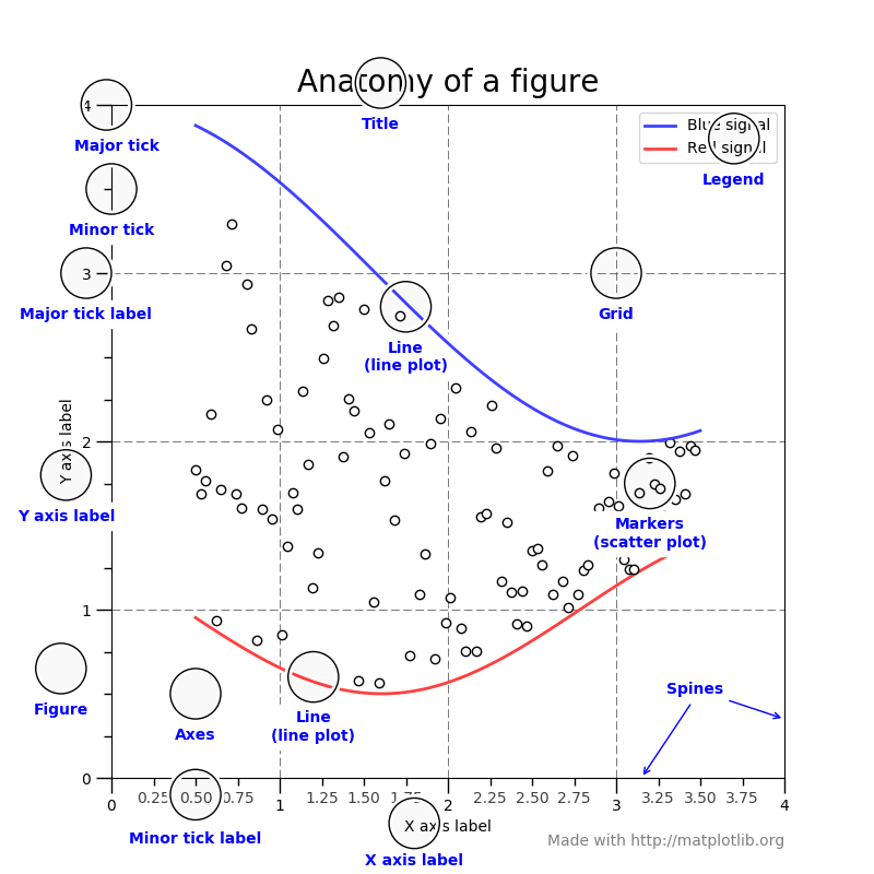
1.1 基本术语
matplotlib 的基本术语可以参考官网中展示的图。
1.2 绘制图形
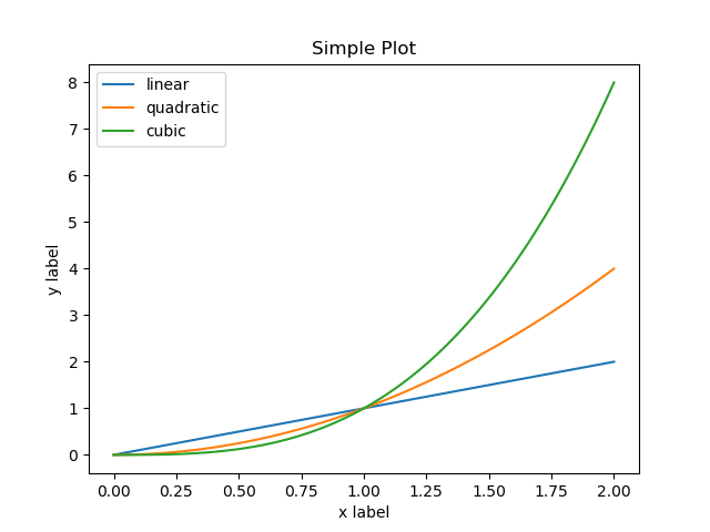
基本画图如下,所有 matplotlib 数据都是使用 numpy 库中的 numpy.array
import matplotlib.pyplot as plt
import numpy as np

filename = "../static/image/2018/10/matplotlib1.png"

x = np.linspace(0, 2, 100)

plt.plot(x, x, label='linear')
plt.plot(x, x**2, label='quadratic')
plt.plot(x, x**3, label='cubic')

plt.xlabel('x label')
plt.ylabel('y label')

plt.title("Simple Plot")

plt.legend()
plt.savefig(filename)
return filename
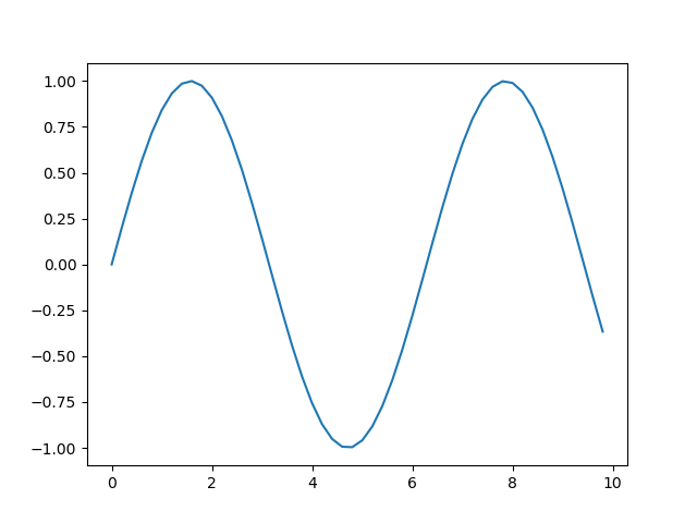
绘制正弦曲线,这里使用 subplots 函数获取子图。
import matplotlib.pyplot as plt
import numpy as np

filename = "../static/image/2018/10/matplotlib2.png"

x = np.arange(0, 10, 0.2)
y = np.sin(x)
fig, ax = plt.subplots()
ax.plot(x, y)

plt.savefig(filename)
return filename
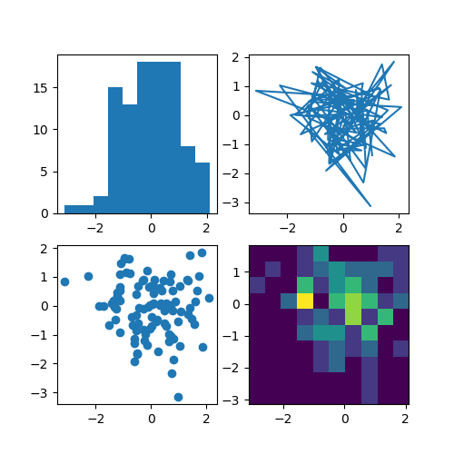
多图并列排版也可以使用 subplots 来实现
import numpy as np
import matplotlib.pyplot as plt
filename = '../static/image/2018/10/matplotlib3.png'

np.random.seed(19680801)
data = np.random.randn(2, 100)

fig, axs = plt.subplots(2, 2, figsize=(5, 5))
axs[0, 0].hist(data[0])
axs[1, 0].scatter(data[0], data[1])
axs[0, 1].plot(data[0], data[1])
axs[1, 1].hist2d(data[0], data[1])

plt.savefig(filename)
return filename
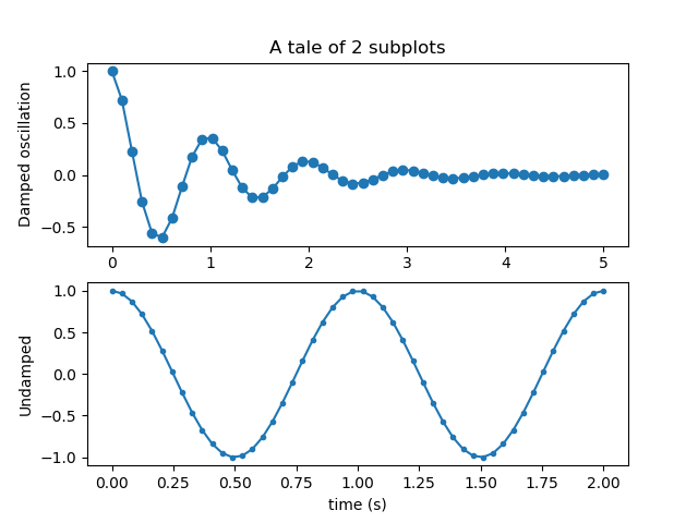
import numpy as np
import matplotlib.pyplot as plt
filename = '../static/image/2018/10/matplotlib4.png'

x1 = np.linspace(0.0, 5.0)
x2 = np.linspace(0.0, 2.0)

y1 = np.cos(2 * np.pi * x1) * np.exp(-x1)
y2 = np.cos(2 * np.pi * x2)

plt.subplot(2, 1, 1)
plt.plot(x1, y1, 'o-')
plt.title('A tale of 2 subplots')
plt.ylabel('Damped oscillation')

plt.subplot(2, 1, 2)
plt.plot(x2, y2, '.-')
plt.xlabel('time (s)')
plt.ylabel('Undamped')

plt.savefig(filename)
return filename
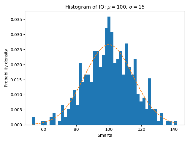
import numpy as np
import matplotlib.pyplot as plt
filename = '../static/image/2018/10/matplotlib5.png'

np.random.seed(19680801)

# example data
mu = 100  # mean of distribution
sigma = 15  # standard deviation of distribution
x = mu + sigma * np.random.randn(437)

num_bins = 50

fig, ax = plt.subplots()

# the histogram of the data
n, bins, patches = ax.hist(x, num_bins, density=1)

# add a 'best fit' line
y = ((1 / (np.sqrt(2 * np.pi) * sigma)) * np.exp(-0.5 * (1 / sigma * (bins - mu))**2))
ax.plot(bins, y, '--')
ax.set_xlabel('Smarts')
ax.set_ylabel('Probability density')
ax.set_title(r'Histogram of IQ: $\mu=100$, $\sigma=15$')

# Tweak spacing to prevent clipping of ylabel
fig.tight_layout()
plt.savefig(filename)
return filename
绘制二维表格
import numpy as np
import matplotlib.pyplot as plt
filename = '../static/image/2018/10/matplotlib6.png'
data = [[ 66386, 174296,  75131, 577908,  32015],
        [ 58230, 381139,  78045,  99308, 160454],
        [ 89135,  80552, 152558, 497981, 603535],
        [ 78415,  81858, 150656, 193263,  69638],
        [139361, 331509, 343164, 781380,  52269]]

columns = ('Freeze', 'Wind', 'Flood', 'Quake', 'Hail')
rows = ['%d year' % x for x in (100, 50, 20, 10, 5)]

values = np.arange(0, 2500, 500)
value_increment = 1000

# Get some pastel shades for the colors
colors = plt.cm.BuPu(np.linspace(0, 0.5, len(rows)))
n_rows = len(data)

index = np.arange(len(columns)) + 0.3
bar_width = 0.4

# Initialize the vertical-offset for the stacked bar chart.
y_offset = np.zeros(len(columns))

# Plot bars and create text labels for the table
cell_text = []
for row in range(n_rows):
    plt.bar(index, data[row], bar_width, bottom=y_offset, color=colors[row])
    y_offset = y_offset + data[row]
    cell_text.append(['%1.1f' % (x / 1000.0) for x in y_offset])
# Reverse colors and text labels to display the last value at the top.
colors = colors[::-1]
cell_text.reverse()

# Add a table at the bottom of the axes
the_table = plt.table(cellText=cell_text,
                      rowLabels=rows,
                      rowColours=colors,
                      colLabels=columns,
                      loc='bottom')

# Adjust layout to make room for the table:
plt.subplots_adjust(left=0.2, bottom=0.2)

plt.ylabel("Loss in ${0}'s".format(value_increment))
plt.yticks(values * value_increment, ['%d' % val for val in values])
plt.xticks([])
plt.title('Loss by Disaster')
plt.savefig(filename)
return filename

1.3 绘制数学函数图像
import numpy as np
import matplotlib.pyplot as plt
import math
filename = '../static/image/2019/02/image081008.png'

def math_plot(x, y, filename):
  fig = plt.figure()
  ax = fig.add_subplot(1, 1, 1)
  # Move left y-axis and bottim x-axis to centre, passing through (0,0)
  ax.spines['left'].set_position('center')
  ax.spines['bottom'].set_position('center')

  # Eliminate upper and right axes
  ax.spines['right'].set_color('none')
  ax.spines['top'].set_color('none')

  # Show ticks in the left and lower axes only
ax.xaxis.set_ticks_position('bottom')
  ax.yaxis.set_ticks_position('left')

  plt.plot(x, y)
  plt.savefig(filename)


x = np.linspace(-3, 3, 500)
y = [t if t > 0 else 0.1 * t for t in x]
math_plot(x, y, filename)

return filename